Problem setting
Newton's method, which is an old numerical approximation technique that could be used to find the roots of complex polynomials and any differentiable function. We'll code it up in 10 lines of Python in this post.
Let's say we have a complicated polynomial:
$latex f(x)=6x^5-5x^4-4x^3+3x^2 $
and we want to find its roots. Unfortunately we know from the Galois theory that there is no formula for a 5th degree polynomial so we'll have to use numeric methods. Wait a second. What's going on? We all learned the quadratic formula in school, and there are formulas for cubic and quartic polynomials, but Galois proved that no such "root-finding" formula exist for fifth or higher degree polynomials, that uses only the usual algebraic operations (addition, subtraction, multiplication, division) and application of radicals (square roots, cube roots, etc).
Bit more maths context
Some nice guys pointed out on reddit that I didn't quite get the theory right. Sorry about that, I'm no mathematician by any means. It turns out that this polynomial could be factored into $latex x^2(x-1)(6x^2 + x - 3)$ and solved with traditional cubic formula.
Also the theorem I referred to is the Abel-Ruffini Theorem and it only applies to the solution to the general polynomial of degree five or greater. Nonetheless the example is still valid, and demonstrates how would you apply Newton's method, to any polynomial, so let's crack on.
Simplest way to solve it
So in these cases we have to resort to numeric linear approximation. A simple way would be to use the intermediate value theorem, which states that if $latex f(x)$ is continuous on $latex [a,b]$ and $latex f(a) < y< f(b)$, then there is an $latex x$ between $latex a$ and $latex b$ so that $latex f(x)=y$.
We could exploit this by looking for an $latex x_1$ where $latex f(x_1)>0$ and an $latex x_2$ where $latex f(x_2)<0$, and then we could be certain that $latex f(x)=0$ must be between $latex x_1$ and $latex x_2$. So we could check $latex x_3=\frac{x_2-x_1}{2}$, and find that $latex f(x_3)$ will be positive, then continue with$latex x_4=\frac{x_2-x_3}{2}$ which would be negative and our proposed $latex x_n$ would become closer and closer to $latex f(x_n)=0$. This method however can be pretty slow, so Newton devised a better way to speed things up (when it works).
How Newton solved it
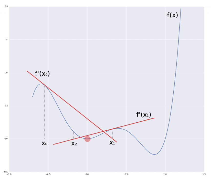
If you look at the figure below, you'll see the plot of our polynomial. It has three roots at 0, 1, and somewhere in-between. So how do we find these?
In Newton's method we take a random point $latex f(x_0)$, then draw a tangent line through $latex x_0, f(x_0)$, using the derivative $latex f'(x_0)$. The point $latex x_1$ where this tangent line crosses the $latex x$ axis will become the next proposal we check. We calculate the tangent line at $latex f'(x_1)$ and find $latex x_2$. We carry on, and as we do $latex |f(x_n)| \to 0$, or in other words we can make our approximation as close to zero as we want, provided we are willing to continue with the number crunching. Using the fact that the slope of tangent (by the definition of derivatives) at $latex x_n$ is $latex f'(x_n)$ we can derive the formula for $latex x_{n+1}$, i.e. where the tangent crosses the $latex x$ axis:
$latex x_{n+1}=x_n-\frac{f(x_n)}{f'(x_n)}$
Code
With all this in mind it's easy to write an algorithm that approximates $f(x)=0$ with arbitrary error $latex \varepsilon$. Obviously in this example depending on where we start $latex x_0$ we might find different roots.
1
2
3
4
5
6
7
8
9
10
def dx(f, x):
    return abs(0-f(x))

def newtons_method(f, df, x0, e):
    delta = dx(f, x0)
    while delta > e:
        x0 = x0 - f(x0)/df(x0)
        delta = dx(f, x0)
    print 'Root is at: ', x0
    print 'f(x) at root is: ', f(x0)
There you go, we’are done in 10 lines (9 without the blank line), even less without the print statements.
In use
So in order to use this, we need two functions, $latex f(x)$ and $latex f'(x)$. For this polynomial these are:
1
2
3
4
5
def f(x):
    return 6*x**5-5*x**4-4*x**3+3*x**2

def df(x):
    return 30*x**4-20*x**3-12*x**2+6*x
Now we can simply find the three roots with:
1
2
3
4
5
6
7
8
9
10
x0s = [0, .5, 1]
for x0 in x0s:
    newtons_method(f, df, x0, 1e-5)

# Root is at:  0
# f(x) at root is:  0
# Root is at:  0.628668078167
# f(x) at root is:  -1.37853879978e-06
# Root is at:  1
# f(x) at root is:  0
Summary
All of the above code, and some additional comparison test with the scipy.optimize.newton method can be found in this Gist. And don’t forget, if you find it too much trouble differentiating your functions, just use SymPy, I wrote about it here.
Newton’s method is pretty powerful but there could be problems with the speed of convergence, and awfully wrong initial guesses might make it not even converge ever, see here. Nonetheless I hope you found this relatively useful.. Let me know in the comments.
Comments