BorutaPy

Quick summary

There’s a pretty clever all-relevant feature selection method, which was conceived by Witold R. Rudnicki and developed by Miron B. Kursa at the ICM UW. Here is the publication.

While working on my PhD project I read their paper, really liked the method, but didn’t quite like how slow it was. It’s based on R’s Random Forest implementation which runs only on a single core.

On the other hand, I knew that the core dev team working at scikit-learn on the Random Forest Classifier has made an incredible job at optimizing its performance making it the fastest implementation currently available. So I thought I’d re-implement the algorithm in Python. It runs pretty fast now, and has a scikit-learn like interface, so you can call fit(), transform() and fit_transform() on it. You can check it out on my GitHub.

Miron kindly agreed to benchmark it against his original version so it might get modified, but in the meanwhile please feel free to use it and let me know what you think!

Background

What’s feature selection?

In many data analysis and modelling projects we end up with hundreds or thousands of collected features. Even worse, sometimes we have way more features than samples. It is a setting that is becoming increasingly common, at least in biomedical sciences for sure. This is called a small n large p situation, which pretty much means you’re left with regularized (preferably lasso) regression techniques if you want to avoid massively over-fitting your data.

But fortunately most of the time not all your variables are interesting or relevant to the stuff you’re trying to understand/model. So you can try to devise clever ways to select the important ones and incorporate only those into your model, this is called feature selection and there are loads of published methods floating around.

Doing the simple way

Probably the easiest way to go about feature selection, is to do some univariate test on each of your features relating it to the predicted outcome, and select the ones that do pretty well based on some obscenely arbitrary measure or some simple statistical test.

This is simple and quick, but also univariate, which means it’s probably only useful if you can guarantee that all of your features are completely independent. Unless you are modelling some simulated toy dataset this is never the case.

In fact, one of the main reasons doing science is so incredibly hard is because of the many intricate unknown relationships between your measured variables and other confounders you haven’t even thought of. OK, so what else?

Going multivariate

Well, you can do feature selection using a multivariate model, like Support Vector Machine. First you fit it to your data and get the weights it assigns to each of your features. Then you can recursively get rid of features in each round which didn’t do too well, until you reach some predefined end point when you stop.

This is definitely slower, but it is also presumably better as it’s multivariate meaning it will attempt to weigh in the various relationships between your predictive variables and select a set of features that together explain a lot of the variance in your data. On the other hand it is quite arbitrary when you stop, or how many features you get rid off at each round. I hear you say, you can do an exhaustive grid search on these hyper-parameters, or include some cross-validation to make sure you stop at the right point.

But even then, this method essentially is maximizing a regressor’s or classifier’s performance by selecting an exceedingly pruned version of your input data matrix. This might be a good a thing, but it can also throw away a number of important features.

How is Boruta different?

Boruta is an all-relevant feature selection method. It tries to capture all the important, interesting features you might have in your dataset with respect to an outcome variable.

Boruta is an all relevant feature selection method, while most other are minimal optimal; this means it tries to find all features carrying information usable for prediction, rather than finding a possibly compact subset of features on which some classifier has a minimal error.
Miron B. Kursa

This makes it really well suited for biomedical data analysis, where we regularly collect measurements of thousands of features (genes, proteins, metabolites, microbiomes in your gut, etc), but we have absolutely no clue about which one is important in relation to our outcome variable, or where should we cut off the decreasing “importance function” of these.

As with so many great algorithms the idea behind Boruta is really simple. First, we duplicate our dataset, and shuffle the values in each column, these are called shadow features.

Then we train a classifier on our dataset, such that we get importances for each of our features. Tree ensemble methods such as Random Forest, Gradient Boosted Trees, and the Extra Trees Classifiers are really great not only because they can capture non-linear highly intricate relationships between your predictors, but also because they tend to handle the small n large p situation rather well.

Why should you care? For a start, when you try to understand the phenomenon that made your data, you should care about all factors that contribute to it, not just the bluntest signs of it in context of your methodology (yes, minimal optimal set of features by definition depends on your classifier choice).
Miron B. Kursa

There is quite a lot of discussion about whether these methods can truly overfit your training data, but generally it is accepted that even if they do, this happens much later with them than with many other machine learning algorithms.

Back to the Boruta. So we train one of these ensemble methods on our merged training data and shadow features (see the image below). Then we get the relative importance of each feature from the ensemble method: higher means better or more important.

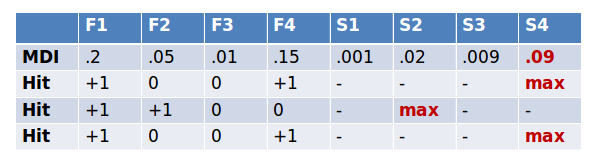
Then we check for each of our real features if they have higher importance than the best of the shadow features. If they do, we record this in a vector (these are called a hits) and continue with another iteration. After a predefined set of iterations we end up with a table of these hits.

At every iteration we check if a given feature is doing better then expected than random chance. We do this by simply comparing the number of times a feature did better than the shadow features using a binomial distribution.

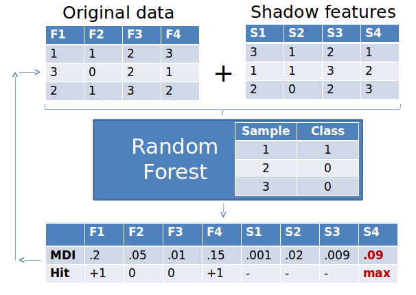
In the case of feature #1 in the table below, out of 3 runs it did better than the best of shadow features 3 times. So we calculate a p-value  using the binomial distribution, k=3, n=3, p=0.5. As we do this for thousands of features we need to correct for multiple testing. The original method uses the rather conservative Bonferroni correction for this. We say a feature is confirmed to be important if its corrected p-value is lower than 0.01.

Then we remove its column from the original data matrix and continue with another iteration.

Conversely if a feature hasn’t been recorded as a hit in say 15 iterations, we reject it and also remove it from the original matrix. After a set number of iterations (or if all the features have been either confirmed or rejected) we stop.

For all the parameters and options please check the GitHub site and the documentation for more details.

Python implementation

The Python version requires numpy, scipy, scikit-learn and bottleneck, so you’ll need to install these before trying it, but then you can simply apply it to your dataset like this:

import pandas
from sklearn.ensemble import RandomForestClassifier
from boruta_py import boruta_py

# load X and y
X = pd.read_csv('my_X_table.csv', index_col=0).values
y = pd.read_csv('my_y_vector.csv', index_col=0).values

# define random forest classifier, with utilising all cores and
# sampling in proportion to y labels
forest = RandomForestClassifier(n_jobs=-1, class_weight='auto')

# define Boruta feature selection method
feat_selector = boruta_py.BorutaPy(forest, n_estimators='auto', verbose=2)

# find all relevant features
feat_selector.fit(X, y)

# check selected features
feat_selector.support_

# check ranking of features
feat_selector.ranking_

# call transform() on X to filter it down to selected features
X_filtered = feat_selector.transform(X)

Again, all of the parameters, attributes and methods are documented with docstrings so grab a copy or fork it and let me know what you think!